
gpsview.py plots GPS satellite signal-to-noise ratio values read from files of NMEA sentences generated by a GPS receiver monitoring the signal from a GNSS re-transmitter and recorded by the companion program gpsnmea.py.
![]()
![]()
Some re-transmitters.
At the PASSCAL Instrument Center in Socorro we have several GNSS re-transmitters. All of our seismic recording equipment relies on the GPS system for accurate timing. Sometimes the position of the recorders in the field are also used to measure things like the movement of a glacier or iceberg that the station is sitting on.
The receiver keeping an eye on the transmitter.
While it is easy to see if a GNSS receiver in a recorder and, usually,
the attached antenna are working, it wasn't possible to see how well
the repeaters in the labs were working. After a few suspicious bench
test results where there were GPS problems I came up with the idea of
using small GPS receivers to watch the repeaters by placing the
receivers near the repeaters and recording the NMEA sentences
generated by the receivers each second.
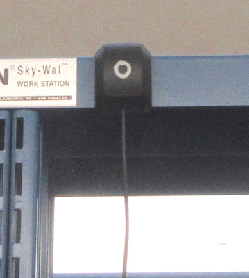
Above is a G-MOUSE GNSS receiver. It is powered by a USB port on one
of our bench PCs. Inside it is a u-Blox GNSS receiver. The program
gpsnmea.py, runs on the bench PC and collects the 5 or 6 NEMA
sentences that are generated by the receiver each second. The
sentences are grouped into one file per UT day. Each file is about
30MBs in size.
The receivers are configured with the u-Blox u-Center software to only
receive the GPS satellites. The geostationary satellites used by the
GPS system and other constellations, such as GLONASS, would skew the
results.
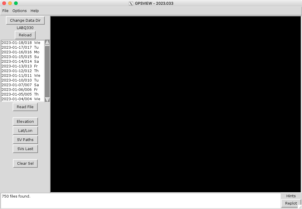
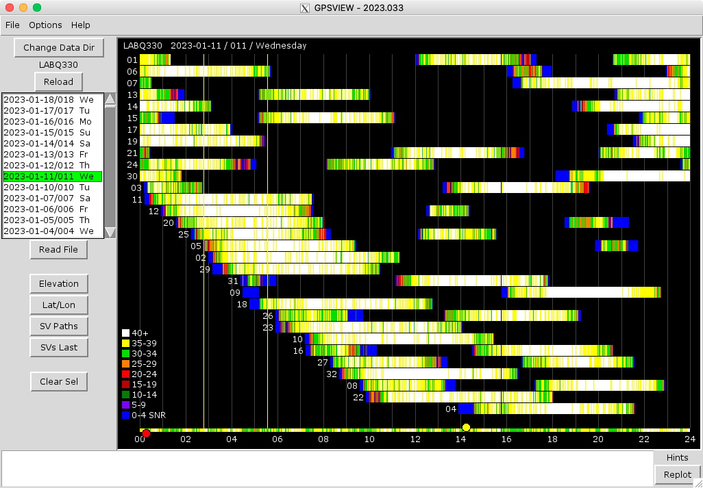
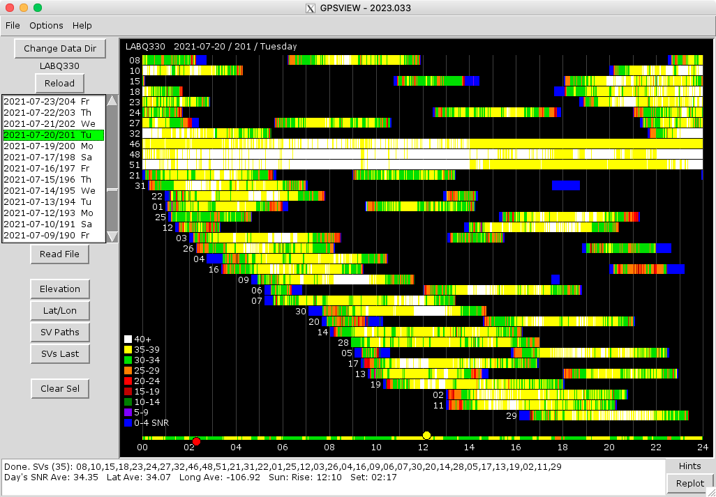
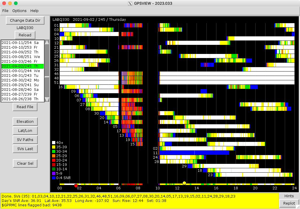
Above is the main display of the program. It has a list of dates on
the left side each of which are associated with a daily file of NMEA
sentences. The label above the list of files indicates that the
dates/files are in the data directory LABQ330.
Additional G-MOUSE receivers and additional instances of gpsnmea.py
writing to different directories can be set up on a computer to
collect the sentences for each re-transmitter to be monitored. The
different data directories may be selected with the Change Data Dir
button.
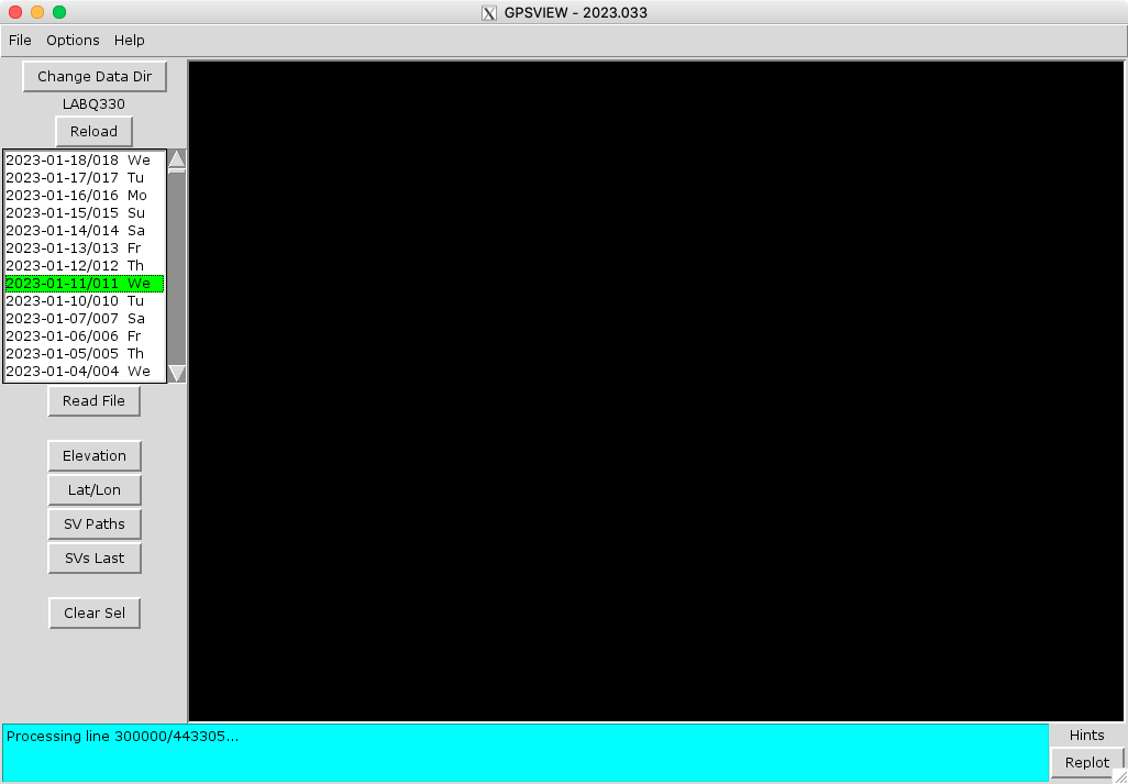
Reading the data from one of the day files is started by double-clicking on one of the dates or selecting one and clicking the Read File button below the list.

When reading and processing the file is finished the information will
be plotted showing horizontal lines that are the SNR values for each
satellite as they progress across the sky during one UT day. The
numbers at the beginning of each row are the NMEAID numbers, which
relate to the Space Vehicle Numbers for each satellite. Where there is
information is where each satellite is above the horizon, and where
the plots are blank is where the satellites are below. From the plot
above it can be seen that satellite 24 appeared in the sky three times
during the day.
The plot across the bottom is the average SNR of all visible
satellites above the plot at each point in time.
The red dot is the time of sunset, and the yellow dot is sunrise. The
Sun being up or down doesn't make a lot of difference to GPS signals,
sorta. The signals are affected by changes in the ionosphere, which
can degrade the position solution, but changes in SNR will probably
not be visible in this program. The Lat Ave and Long Ave values in the
notifications area are the position used to make the rise/set
calculations. If that position information is not correct then the
dots will not be in the right place. If there is only a yellow dot it
means that the Sun was up all day. If there is just a red dot it means
that the Sun was set all day.
The Replot button will redraw the plots without having to re-read the
day file. For example this could be used after resizing the main
window.
The vertical thin black line running through all of the plots just
before 1600 was probably when the gpsnmea.py was stopped for a short
time maybe when the lab computer was rebooted.
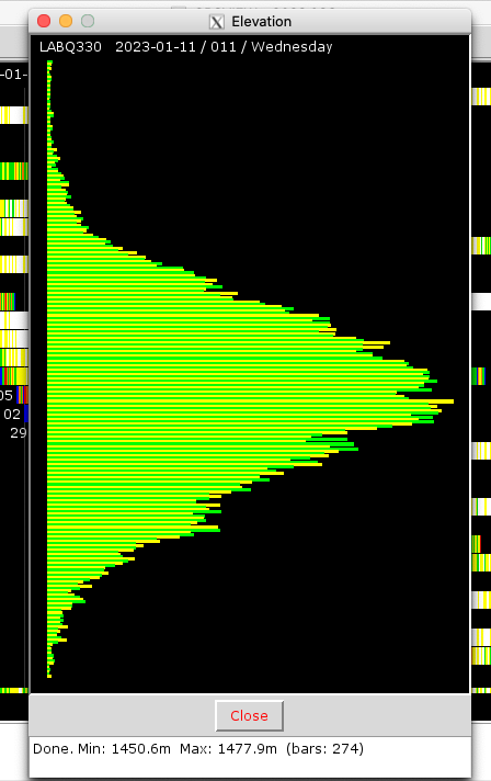
The Elevation button brings up a plot that looks like a histogram of
all of the elevation readings from the previously read daily NMEA
file. It's not quite a histogram in that the y-axis is not graduated
in regular intervals. The bars are a count of the number of times an
elevation shows up. If there are no points for a given elevation there
won't be a blank bar, that elevation will just be skipped over.
Each bar can be clicked on more more details about the elevation it
represents.
GPS position information is not normally stable for simple GPS
receivers. It wanders a bit. The quality can be affected by anything
from atmospheric conditions, antenna and receiver quality,
constellation position of satellites, and objects blocking receiver
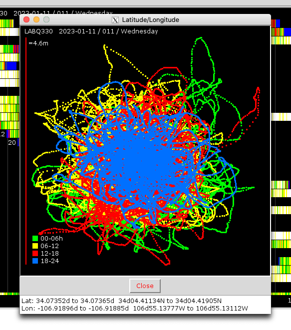
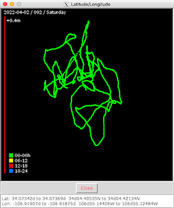
signals. The Lat/Lon button produces a plot that shows the recorded
position for each second.
The plot is colored so that every six hours is a different
color. Down the left side of the plot is a 'maximum width and
height' bar that shows the maximum error of all of the points
in both latitude and longitude. On a good day the error might
be around three meters. On a bad day, without equipment
problems, it may be in the tens of meters.
The plot is not corrected for latitude as the position gets
closer to the poles. It is the same number of degrees in X and
Y.
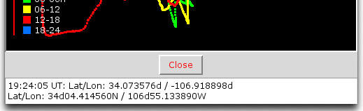
Each dot can be clicked to reveal the latitude, longitude and time that position was recorded. The values are displayed in the two different formats just for fun.
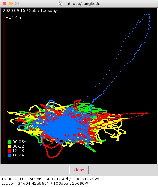
Sometimes things get a little crazy.
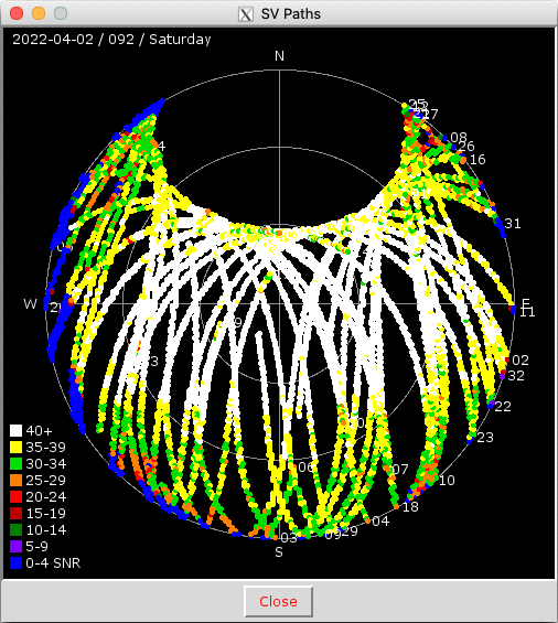
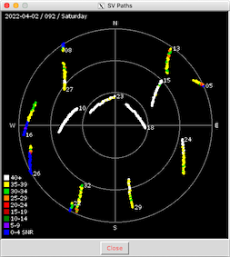
The SV Paths button brings up a plot that shows the path of each satellite throughout the day. Straight up is in the center and the horizon around the edge. From the plot we can see that the SNR improves when the satellites are high in the sky and start to go down towards the horizon. Socorro has a few mountains to the west of town and the plot above shows that with the SNR values staying low when the satellites are about ten to twelve degrees above the horizon.

The SVs Last button simply shows the position and SNR values of the satellites at the "latest" time of the day plotted. Usually when using the system during bench testing you want to know what is going on right now. This makes it easy to find out.
Shift-clicking, twice, on the main plot allows you to select a
sub-set of the day's data. Selecting the Elevation, Lat/Lon,
or SV Paths button will plot the same information as before,
but only during the selected time range.
Shift-clicking on the extreme left side of the main plot, or
clicking the Clear Sel button will erase the selection lines.

Less time, fewer points.
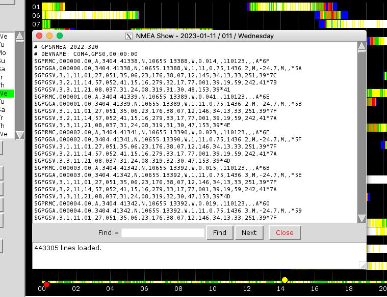
Selecting and then shift-clicking on one of the dates will open the corresponding NMEA sentence file for inspection.
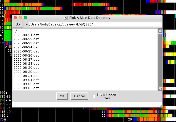
The Change Data Dir button, or the menu command File | Change Data Directory... command will bring up a file selection dialog box to allow navigating to different sub-directories associated with the running of multiple copies of gpsnmea.py.
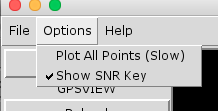
The Options menu contains two items.
On the main plot usually defaults to about 800 or so pixels to plot up
to 86,400 points. That means 100 points will plotted on top of each
other per pixel. That wastes time. Not selecting the option Plot All
Points (Slow), will speed up plotting significantly by not drawing all
of those redundant points. This option is available mostly as a
curiosity.
The Show SNR Key simply toggles showing or not showing the color key
that associates the plot colors with the SNR values on the main
plot. During the early part of the day the satellite plots will extend
all of the way to the bottom of the plot area on the left side and the
key will write over some of the plots.
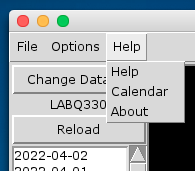
The Help menu contains the usual suspects.
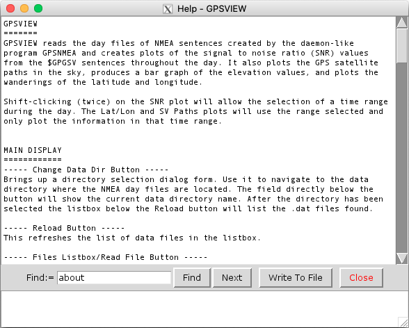
Built-in help.

The standard three-month calendar as in other programs of mine.

The usual About dialog.
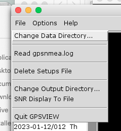
The File menu item Change Data Directory accomplishes the same function as the Change Data Dir button.

The Read gpsnmea.log command brings up a simple text display form. The
gpsnmea.py program collects the NMEA sentences from the GPS receiver
and writes status messages to this file.
The setups file is used to save the various program settings, so they
can be recalled the next time the program is started. This command
erases this file to restore all of the default settings.
The program is capable of producing a .png image of the main display
area. Change Output Directory... is used to navigate to a place to
save the file, and SNR Display To File is used to make the file. In
some cases this may not work, because of the way it is done.
Screenshotting using the OS method is a more reliable way.
One fine day.
Not so fine. New Mexico has thunderstorms. Above was the result of one lightning strike that hit close to the building.
The strike didn't hit the antenna on the roof, but it took out an antenna signal splitter that was upstream of the re-transmitter and sitting on top of some shelves in the lab. The picture above shows when I figured out it was the splitter and it was removed. We didn't need it anymore anyway.
As if lightning isn't enough. White Sands Missile Range (WSMR), the Trinity Site and all of that, is just a little ways down the road from Socorro. A few times a year WSMR reserves some time and conducts tests on/with the GPS system. Jamming, spoofing...the usual. We are almost always in the line of fire. Their testing usually happens during the night. Having the gpsview.py/gpsnmea.py monitoring system helps to explain those times when our GPS receivers mysteriously lose lock during bench tests. One of those times was the driving force behind its creation.
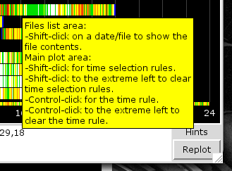
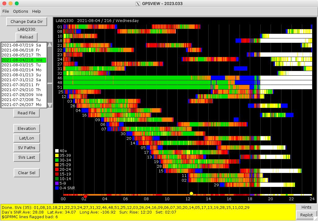
Added a Hints tooltip as the number of features creeped.
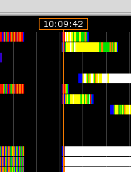
A control-click on the main plot will show a rule indicating the time of the day at that point. The time shown may not be entirely accurate. 86,400 seconds get crammed into a few hundred pixels, so each pixel represents many seconds or even minutes depending on how wide the plot area is stretched.
2023-02-06